7. Test with ICNet Pre-trained Models for Multi-Human Parsing

This is a quick demo of using GluonCV ICNet model for multi-human parsing on real-world images. Please follow the installation guide to install MXNet and GluonCV if not yet.

import mxnet as mx
from mxnet import image
from mxnet.gluon.data.vision import transforms
import gluoncv
# using cpu
ctx = mx.cpu(0)

Prepare the image

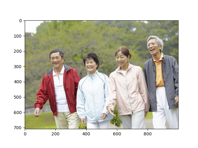
Let’s first download the example image,

url = 'https://raw.githubusercontent.com/dmlc/web-data/master/gluoncv/segmentation/mhpv1_examples/1.jpg'
filename = 'mhp_v1_example.jpg'
gluoncv.utils.download(url, filename, True)

Out:

Downloading mhp_v1_example.jpg from https://raw.githubusercontent.com/dmlc/web-data/master/gluoncv/segmentation/mhpv1_examples/1.jpg...

  0%|          | 0/84 [00:00<?, ?KB/s]
85KB [00:00, 22401.25KB/s]

Then we load the image and visualize it,

img = image.imread(filename)

from matplotlib import pyplot as plt
plt.imshow(img.asnumpy())
plt.show()

We normalize the image using dataset mean and standard deviation,

from gluoncv.data.transforms.presets.segmentation import test_transform
img = test_transform(img, ctx)

Load the pre-trained model and make prediction

Next, we get a pre-trained model from our model zoo,

model = gluoncv.model_zoo.get_model('icnet_resnet50_mhpv1', pretrained=True)

Out:

Downloading /root/.mxnet/models/icnet_resnet50_mhpv1-873d381a.zip from https://apache-mxnet.s3-accelerate.dualstack.amazonaws.com/gluon/models/icnet_resnet50_mhpv1-873d381a.zip...

  0%|          | 0/185766 [00:00<?, ?KB/s]
  0%|          | 93/185766 [00:00<04:42, 658.06KB/s]
  0%|          | 508/185766 [00:00<01:32, 2001.85KB/s]
  1%|1         | 2188/185766 [00:00<00:28, 6517.20KB/s]
  4%|3         | 6731/185766 [00:00<00:09, 18809.92KB/s]
  6%|6         | 12029/185766 [00:00<00:06, 28250.37KB/s]
 10%|#         | 19190/185766 [00:00<00:04, 41210.15KB/s]
 14%|#3        | 25098/185766 [00:00<00:03, 44889.34KB/s]
 17%|#6        | 31235/185766 [00:00<00:03, 49693.61KB/s]
 20%|#9        | 37120/185766 [00:01<00:02, 50269.65KB/s]
 24%|##4       | 44829/185766 [00:01<00:02, 57976.30KB/s]
 28%|##8       | 52163/185766 [00:01<00:02, 56537.32KB/s]
 32%|###1      | 58711/185766 [00:01<00:02, 56797.25KB/s]
 36%|###5      | 66022/185766 [00:01<00:01, 61255.17KB/s]
 39%|###8      | 72258/185766 [00:01<00:02, 48588.26KB/s]
 42%|####1     | 77576/185766 [00:01<00:02, 41909.18KB/s]
 44%|####4     | 82196/185766 [00:02<00:02, 39298.01KB/s]
 47%|####6     | 86968/185766 [00:02<00:03, 31731.64KB/s]
 49%|####9     | 91310/185766 [00:02<00:02, 33079.14KB/s]
 51%|#####1    | 94943/185766 [00:02<00:02, 33688.28KB/s]
 54%|#####4    | 100635/185766 [00:02<00:02, 38440.99KB/s]
 56%|#####6    | 104748/185766 [00:02<00:02, 34234.61KB/s]
 59%|#####8    | 109117/185766 [00:02<00:02, 36477.29KB/s]
 61%|######1   | 113983/185766 [00:02<00:01, 39560.41KB/s]
 64%|######3   | 118156/185766 [00:03<00:01, 39849.44KB/s]
 66%|######5   | 122296/185766 [00:03<00:02, 29446.38KB/s]
 70%|######9   | 129353/185766 [00:03<00:01, 38586.30KB/s]
 74%|#######3  | 137048/185766 [00:03<00:01, 47208.52KB/s]
 78%|#######7  | 144094/185766 [00:03<00:00, 53087.43KB/s]
 82%|########1 | 151780/185766 [00:03<00:00, 59407.10KB/s]
 85%|########5 | 158516/185766 [00:03<00:00, 61595.54KB/s]
 89%|########9 | 165659/185766 [00:03<00:00, 64368.41KB/s]
 93%|#########2| 172585/185766 [00:03<00:00, 65666.15KB/s]
 97%|#########6| 179338/185766 [00:04<00:00, 63582.55KB/s]
100%|##########| 185766/185766 [00:04<00:00, 44385.60KB/s]

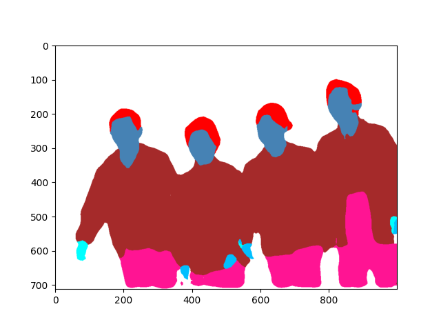
We directly make semantic predictions on the image,

output = model.predict(img)
predict = mx.nd.squeeze(mx.nd.argmax(output, 1)).asnumpy()

In the end, we add color pallete for visualizing the predicted mask,

from gluoncv.utils.viz import get_color_pallete
import matplotlib.image as mpimg
mask = get_color_pallete(predict, 'mhpv1')
mask.save('output.png')
mmask = mpimg.imread('output.png')
plt.imshow(mmask)
plt.show()