Note
Click here to download the full example code
04. Train SSD on Pascal VOC dataset
This tutorial goes through the basic building blocks of object detection provided by GluonCV. Specifically, we show how to build a state-of-the-art Single Shot Multibox Detection [Liu16] model by stacking GluonCV components. This is also a good starting point for your own object detection project.
Hint
You can skip the rest of this tutorial and start training your SSD model right away by downloading this script:
Example usage:
Train a default vgg16_atrous 300x300 model with Pascal VOC on GPU 0:
python train_ssd.py
Train a resnet50_v1 512x512 model on GPU 0,1,2,3:
python train_ssd.py --gpus 0,1,2,3 --network resnet50_v1 --data-shape 512
Check the supported arguments:
python train_ssd.py --help
Dataset
Please first go through this Prepare PASCAL VOC datasets tutorial to setup Pascal VOC dataset on your disk. Then, we are ready to load training and validation images.
from gluoncv.data import VOCDetection
# typically we use 2007+2012 trainval splits for training data
train_dataset = VOCDetection(splits=[(2007, 'trainval'), (2012, 'trainval')])
# and use 2007 test as validation data
val_dataset = VOCDetection(splits=[(2007, 'test')])

print('Training images:', len(train_dataset))
print('Validation images:', len(val_dataset))
Out:
Training images: 16551
Validation images: 4952
Data transform
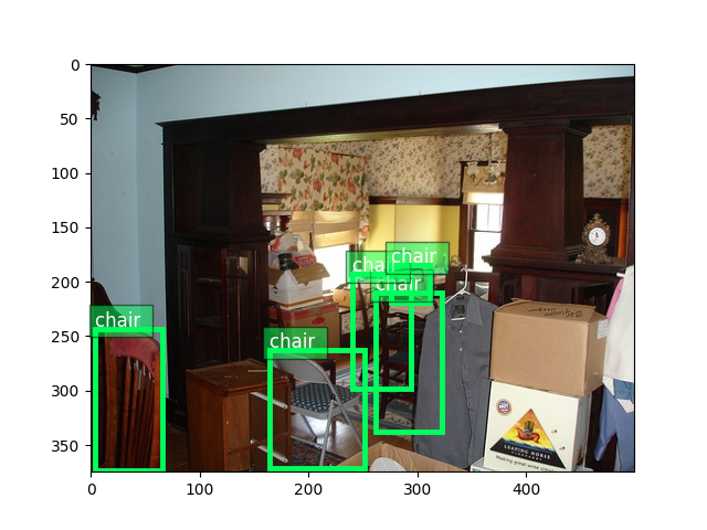
We can read an image-label pair from the training dataset:
train_image, train_label = train_dataset[0]
bboxes = train_label[:, :4]
cids = train_label[:, 4:5]
print('image:', train_image.shape)
print('bboxes:', bboxes.shape, 'class ids:', cids.shape)
Out:
image: (375, 500, 3)
bboxes: (5, 4) class ids: (5, 1)
Plot the image, together with the bounding box labels:
from matplotlib import pyplot as plt
from gluoncv.utils import viz

ax = viz.plot_bbox(
    train_image.asnumpy(),
    bboxes,
    labels=cids,
    class_names=train_dataset.classes)
plt.show()
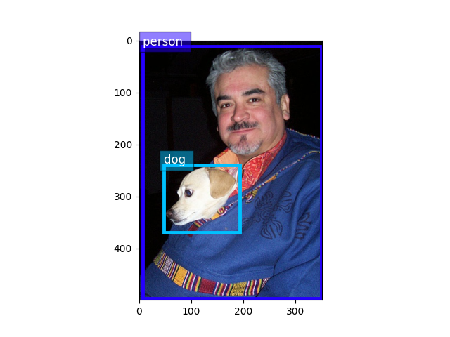
Validation images are quite similar to training because they were basically split randomly to different sets
val_image, val_label = val_dataset[0]
bboxes = val_label[:, :4]
cids = val_label[:, 4:5]
ax = viz.plot_bbox(
    val_image.asnumpy(),
    bboxes,
    labels=cids,
    class_names=train_dataset.classes)
plt.show()
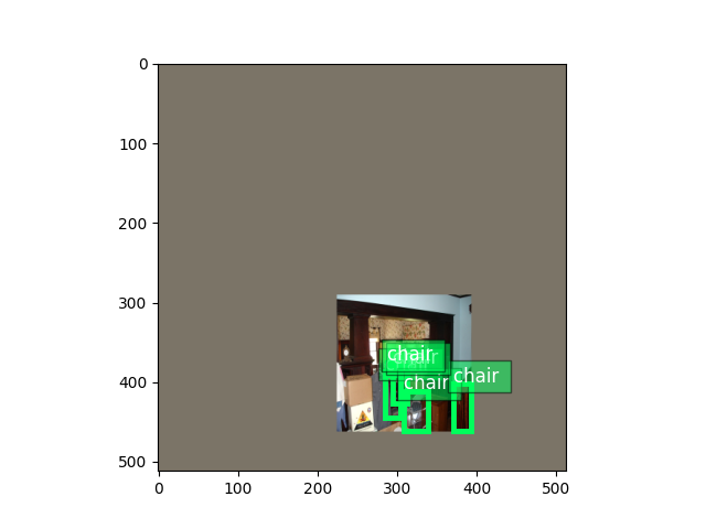
For SSD networks, it is critical to apply data augmentation (see explanations in paper [Liu16]). We provide tons of image and bounding box transform functions to do that. They are very convenient to use as well.
from gluoncv.data.transforms import presets
from gluoncv import utils
from mxnet import nd
width, height = 512, 512  # suppose we use 512 as base training size
train_transform = presets.ssd.SSDDefaultTrainTransform(width, height)
val_transform = presets.ssd.SSDDefaultValTransform(width, height)
utils.random.seed(233) # fix seed in this tutorial
apply transforms to train image
train_image2, train_label2 = train_transform(train_image, train_label)
print('tensor shape:', train_image2.shape)
Out:
tensor shape: (3, 512, 512)
Images in tensor are distorted because they no longer sit in (0, 255) range. Let’s convert them back so we can see them clearly.
train_image2 = train_image2.transpose(
    (1, 2, 0)) * nd.array((0.229, 0.224, 0.225)) + nd.array((0.485, 0.456, 0.406))
train_image2 = (train_image2 * 255).clip(0, 255)
ax = viz.plot_bbox(train_image2.asnumpy(), train_label2[:, :4],
                   labels=train_label2[:, 4:5],
                   class_names=train_dataset.classes)
plt.show()
apply transforms to validation image
val_image2, val_label2 = val_transform(val_image, val_label)
val_image2 = val_image2.transpose(
    (1, 2, 0)) * nd.array((0.229, 0.224, 0.225)) + nd.array((0.485, 0.456, 0.406))
val_image2 = (val_image2 * 255).clip(0, 255)
ax = viz.plot_bbox(val_image2.clip(0, 255).asnumpy(), val_label2[:, :4],
                   labels=val_label2[:, 4:5],
                   class_names=train_dataset.classes)
plt.show()
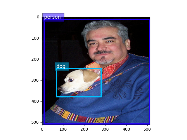
Transforms used in training include random expanding, random cropping, color distortion, random flipping, etc. In comparison, validation transforms are simpler and only resizing and color normalization is used.
Data Loader
We will iterate through the entire dataset many times during training. Keep in mind that raw images have to be transformed to tensors (mxnet uses BCHW format) before they are fed into neural networks. In addition, to be able to run in mini-batches, images must be resized to the same shape.
A handy DataLoader would be very convenient for us to apply different transforms and aggregate data into mini-batches.
Because the number of objects varies a lot across images, we also have
varying label sizes. As a result, we need to pad those labels to the same size.
To deal with this problem, GluonCV provides gluoncv.data.batchify.Pad,
which handles padding automatically.
gluoncv.data.batchify.Stack in addition, is used to stack NDArrays with consistent shapes.
gluoncv.data.batchify.Tuple is used to handle different behaviors across multiple outputs from transform functions.
from gluoncv.data.batchify import Tuple, Stack, Pad
from mxnet.gluon.data import DataLoader

batch_size = 2  # for tutorial, we use smaller batch-size
# you can make it larger(if your CPU has more cores) to accelerate data loading
num_workers = 0

# behavior of batchify_fn: stack images, and pad labels
batchify_fn = Tuple(Stack(), Pad(pad_val=-1))
train_loader = DataLoader(
    train_dataset.transform(train_transform),
    batch_size,
    shuffle=True,
    batchify_fn=batchify_fn,
    last_batch='rollover',
    num_workers=num_workers)
val_loader = DataLoader(
    val_dataset.transform(val_transform),
    batch_size,
    shuffle=False,
    batchify_fn=batchify_fn,
    last_batch='keep',
    num_workers=num_workers)

for ib, batch in enumerate(train_loader):
    if ib > 3:
        break
    print('data:', batch[0].shape, 'label:', batch[1].shape)
Out:
data: (2, 3, 512, 512) label: (2, 3, 6)
data: (2, 3, 512, 512) label: (2, 1, 6)
data: (2, 3, 512, 512) label: (2, 2, 6)
data: (2, 3, 512, 512) label: (2, 1, 6)
SSD Network
GluonCV’s SSD implementation is a composite Gluon HybridBlock (which means it can be exported to symbol to run in C++, Scala and other language bindings. We will cover this usage in future tutorials). In terms of structure, SSD networks are composed of base feature extraction network, anchor generators, class predictors and bounding box offset predictors.
For more details on how SSD detector works, please refer to our introductory tutorial You can also refer to the original paper to learn more about the intuitions behind SSD.
Gluon Model Zoo has a lot of built-in SSD networks. You can load your favorite one with one simple line of code:
Hint
To avoid downloading models in this tutorial, we set pretrained_base=False, in practice we usually want to load pre-trained imagenet models by setting pretrained_base=True.
from gluoncv import model_zoo
net = model_zoo.get_model('ssd_300_vgg16_atrous_voc', pretrained_base=False)
print(net)
Out:
SSD(
  (features): VGGAtrousExtractor(
    (stages): HybridSequential(
      (0): HybridSequential(
        (0): Conv2D(None -> 64, kernel_size=(3, 3), stride=(1, 1), padding=(1, 1))
        (1): Activation(relu)
        (2): Conv2D(None -> 64, kernel_size=(3, 3), stride=(1, 1), padding=(1, 1))
        (3): Activation(relu)
      )
      (1): HybridSequential(
        (0): Conv2D(None -> 128, kernel_size=(3, 3), stride=(1, 1), padding=(1, 1))
        (1): Activation(relu)
        (2): Conv2D(None -> 128, kernel_size=(3, 3), stride=(1, 1), padding=(1, 1))
        (3): Activation(relu)
      )
      (2): HybridSequential(
        (0): Conv2D(None -> 256, kernel_size=(3, 3), stride=(1, 1), padding=(1, 1))
        (1): Activation(relu)
        (2): Conv2D(None -> 256, kernel_size=(3, 3), stride=(1, 1), padding=(1, 1))
        (3): Activation(relu)
        (4): Conv2D(None -> 256, kernel_size=(3, 3), stride=(1, 1), padding=(1, 1))
        (5): Activation(relu)
      )
      (3): HybridSequential(
        (0): Conv2D(None -> 512, kernel_size=(3, 3), stride=(1, 1), padding=(1, 1))
        (1): Activation(relu)
        (2): Conv2D(None -> 512, kernel_size=(3, 3), stride=(1, 1), padding=(1, 1))
        (3): Activation(relu)
        (4): Conv2D(None -> 512, kernel_size=(3, 3), stride=(1, 1), padding=(1, 1))
        (5): Activation(relu)
      )
      (4): HybridSequential(
        (0): Conv2D(None -> 512, kernel_size=(3, 3), stride=(1, 1), padding=(1, 1))
        (1): Activation(relu)
        (2): Conv2D(None -> 512, kernel_size=(3, 3), stride=(1, 1), padding=(1, 1))
        (3): Activation(relu)
        (4): Conv2D(None -> 512, kernel_size=(3, 3), stride=(1, 1), padding=(1, 1))
        (5): Activation(relu)
      )
      (5): HybridSequential(
        (0): Conv2D(None -> 1024, kernel_size=(3, 3), stride=(1, 1), padding=(6, 6), dilation=(6, 6))
        (1): Activation(relu)
        (2): Conv2D(None -> 1024, kernel_size=(1, 1), stride=(1, 1))
        (3): Activation(relu)
      )
    )
    (norm4): Normalize(

    )
    (extras): HybridSequential(
      (0): HybridSequential(
        (0): Conv2D(None -> 256, kernel_size=(1, 1), stride=(1, 1))
        (1): Activation(relu)
        (2): Conv2D(None -> 512, kernel_size=(3, 3), stride=(2, 2), padding=(1, 1))
        (3): Activation(relu)
      )
      (1): HybridSequential(
        (0): Conv2D(None -> 128, kernel_size=(1, 1), stride=(1, 1))
        (1): Activation(relu)
        (2): Conv2D(None -> 256, kernel_size=(3, 3), stride=(2, 2), padding=(1, 1))
        (3): Activation(relu)
      )
      (2): HybridSequential(
        (0): Conv2D(None -> 128, kernel_size=(1, 1), stride=(1, 1))
        (1): Activation(relu)
        (2): Conv2D(None -> 256, kernel_size=(3, 3), stride=(1, 1))
        (3): Activation(relu)
      )
      (3): HybridSequential(
        (0): Conv2D(None -> 128, kernel_size=(1, 1), stride=(1, 1))
        (1): Activation(relu)
        (2): Conv2D(None -> 256, kernel_size=(3, 3), stride=(1, 1))
        (3): Activation(relu)
      )
    )
  )
  (class_predictors): HybridSequential(
    (0): ConvPredictor(
      (predictor): Conv2D(None -> 84, kernel_size=(3, 3), stride=(1, 1), padding=(1, 1))
    )
    (1): ConvPredictor(
      (predictor): Conv2D(None -> 126, kernel_size=(3, 3), stride=(1, 1), padding=(1, 1))
    )
    (2): ConvPredictor(
      (predictor): Conv2D(None -> 126, kernel_size=(3, 3), stride=(1, 1), padding=(1, 1))
    )
    (3): ConvPredictor(
      (predictor): Conv2D(None -> 126, kernel_size=(3, 3), stride=(1, 1), padding=(1, 1))
    )
    (4): ConvPredictor(
      (predictor): Conv2D(None -> 84, kernel_size=(3, 3), stride=(1, 1), padding=(1, 1))
    )
    (5): ConvPredictor(
      (predictor): Conv2D(None -> 84, kernel_size=(3, 3), stride=(1, 1), padding=(1, 1))
    )
  )
  (box_predictors): HybridSequential(
    (0): ConvPredictor(
      (predictor): Conv2D(None -> 16, kernel_size=(3, 3), stride=(1, 1), padding=(1, 1))
    )
    (1): ConvPredictor(
      (predictor): Conv2D(None -> 24, kernel_size=(3, 3), stride=(1, 1), padding=(1, 1))
    )
    (2): ConvPredictor(
      (predictor): Conv2D(None -> 24, kernel_size=(3, 3), stride=(1, 1), padding=(1, 1))
    )
    (3): ConvPredictor(
      (predictor): Conv2D(None -> 24, kernel_size=(3, 3), stride=(1, 1), padding=(1, 1))
    )
    (4): ConvPredictor(
      (predictor): Conv2D(None -> 16, kernel_size=(3, 3), stride=(1, 1), padding=(1, 1))
    )
    (5): ConvPredictor(
      (predictor): Conv2D(None -> 16, kernel_size=(3, 3), stride=(1, 1), padding=(1, 1))
    )
  )
  (anchor_generators): HybridSequential(
    (0): SSDAnchorGenerator(

    )
    (1): SSDAnchorGenerator(

    )
    (2): SSDAnchorGenerator(

    )
    (3): SSDAnchorGenerator(

    )
    (4): SSDAnchorGenerator(

    )
    (5): SSDAnchorGenerator(

    )
  )
  (bbox_decoder): NormalizedBoxCenterDecoder(

  )
  (cls_decoder): MultiPerClassDecoder(

  )
)
SSD network is a HybridBlock as mentioned before. You can call it with an input as:
SSD returns three values, where cids are the class labels,
scores are confidence scores of each prediction,
and bboxes are absolute coordinates of corresponding bounding boxes.
SSD network behave differently during training mode:
In training mode, SSD returns three intermediate values,
where cls_preds are the class predictions prior to softmax,
box_preds are bounding box offsets with one-to-one correspondence to anchors
and anchors are absolute coordinates of corresponding anchors boxes, which are
fixed since training images use inputs of same dimensions.
Training targets
Unlike a single SoftmaxCrossEntropyLoss used in image classification,
the loss used in SSD is more complicated.
Don’t worry though, because we have these modules available out of the box.
To speed up training, we let CPU to pre-compute some training targets.
This is especially nice when your CPU is powerful and you can use -j num_workers
to utilize multi-core CPU.
If we provide anchors to the training transform, it will compute training targets
from mxnet import gluon
train_transform = presets.ssd.SSDDefaultTrainTransform(width, height, anchors)
batchify_fn = Tuple(Stack(), Stack(), Stack())
train_loader = DataLoader(
    train_dataset.transform(train_transform),
    batch_size,
    shuffle=True,
    batchify_fn=batchify_fn,
    last_batch='rollover',
    num_workers=num_workers)
Loss, Trainer and Training pipeline
from gluoncv.loss import SSDMultiBoxLoss
mbox_loss = SSDMultiBoxLoss()
trainer = gluon.Trainer(
    net.collect_params(), 'sgd',
    {'learning_rate': 0.001, 'wd': 0.0005, 'momentum': 0.9})

for ib, batch in enumerate(train_loader):
    if ib > 0:
        break
    print('data:', batch[0].shape)
    print('class targets:', batch[1].shape)
    print('box targets:', batch[2].shape)
    with autograd.record():
        cls_pred, box_pred, anchors = net(batch[0])
        sum_loss, cls_loss, box_loss = mbox_loss(
            cls_pred, box_pred, batch[1], batch[2])
        # some standard gluon training steps:
        # autograd.backward(sum_loss)
        # trainer.step(1)
Out:
data: (2, 3, 512, 512)
class targets: (2, 24656)
box targets: (2, 24656, 4)
This time we can see the data loader is actually returning the training targets for us. Then it is very naturally a gluon training loop with Trainer and let it update the weights.
Please checkout the full training script for complete
implementation.