02. Predict depth from an image sequence or a video with pre-trained Monodepth2 models

This article will demonstrate how to estimate depth from your image sequence or video stream.

Please follow the installation guide to install MXNet and GluonCV if not yet.

First, import the necessary modules.

import os
import argparse
import time
import PIL.Image as pil
import numpy as np

import mxnet as mx
from mxnet.gluon.data.vision import transforms

import gluoncv
from gluoncv.model_zoo.monodepthv2.layers import disp_to_depth

import matplotlib as mpl
import matplotlib.cm as cm
import cv2

# using cpu
ctx = mx.cpu(0)

Prepare the data

In this tutorial, we use one sequence of KITTI RAW datasets as an example. Because the KITTI RAW dataset only provides image sequences, the input format is image sequences in this tutorial.

Follow the command to download example data:

cd ~/.mxnet/datasets/kitti/examples
wget https://s3.eu-central-1.amazonaws.com/avg-kitti/raw_data/2011_09_26_drive_0095/2011_09_26_drive_0095_sync.zip
unzip 2011_09_26_drive_0095_sync.zip

After getting the dataset, we can easily load images with PIL.

data_path = os.path.expanduser("~/.mxnet/datasets/kitti/example/2011_09_26/2011_09_26_drive_0095_sync/image_02/data")

files = os.listdir(os.path.expanduser(data_path))
files.sort()

raw_img_sequences = []
for file in files:
    file = os.path.join(data_path, file)
    img = pil.open(file).convert('RGB')
    raw_img_sequences.append(img)

original_width, original_height = raw_img_sequences[0].size

Loading the model

In this tutorial we feed frames from the image sequences into a depth estimation model, then we could get the depth map of the input frame.

For the model, we use monodepth2_resnet18_kitti_mono_stereo_640x192 as it is accurate and could recover the scaling factor of stereo baseline.

model_zoo = 'monodepth2_resnet18_kitti_mono_stereo_640x192'
model = gluoncv.model_zoo.get_model(model_zoo, pretrained_base=False, ctx=ctx, pretrained=True)

Out:

Downloading /root/.mxnet/models/monodepth2_resnet18_kitti_mono_stereo_640x192-9515c219.zip from https://apache-mxnet.s3-accelerate.dualstack.amazonaws.com/gluon/models/monodepth2_resnet18_kitti_mono_stereo_640x192-9515c219.zip...

  0%|          | 0/70343 [00:00<?, ?KB/s]
  0%|          | 101/70343 [00:00<01:21, 858.14KB/s]
  1%|          | 515/70343 [00:00<00:28, 2419.21KB/s]
  3%|3         | 2181/70343 [00:00<00:08, 7736.56KB/s]
 12%|#1        | 8202/70343 [00:00<00:02, 26380.50KB/s]
 21%|##1       | 14992/70343 [00:00<00:01, 40358.57KB/s]
 32%|###1      | 22197/70343 [00:00<00:00, 50649.36KB/s]
 44%|####4     | 31151/70343 [00:00<00:00, 62972.78KB/s]
 56%|#####5    | 39274/70343 [00:00<00:00, 68660.36KB/s]
 68%|######7   | 47647/70343 [00:00<00:00, 73301.38KB/s]
 80%|########  | 56595/70343 [00:01<00:00, 78242.36KB/s]
 92%|#########1| 64492/70343 [00:01<00:00, 78066.28KB/s]
70344KB [00:01, 57446.53KB/s]

Prediction loop

For each frame, we perform the following steps:

• loading a frame from the image sequence

• pre-process the image

• estimate the disparity for the image

• transfer the disparity to a depth map

• store the depth map to the prediction sequence

min_depth = 0.1
max_depth = 100

# while use stereo or mono+stereo model, we could get real depth value
scale_factor = 5.4
MIN_DEPTH = 1e-3
MAX_DEPTH = 80

feed_height = 192
feed_width = 640

pred_depth_sequences = []
pred_disp_sequences = []
for img in raw_img_sequences:
    img = img.resize((feed_width, feed_height), pil.LANCZOS)
    img = transforms.ToTensor()(mx.nd.array(img)).expand_dims(0).as_in_context(context=ctx)

    outputs = model.predict(img)
    mx.nd.waitall()
    pred_disp, _ = disp_to_depth(outputs[("disp", 0)], min_depth, max_depth)
    t = time.time()
    pred_disp = pred_disp.squeeze().as_in_context(mx.cpu()).asnumpy()
    pred_disp = cv2.resize(src=pred_disp, dsize=(original_width, original_height))
    pred_disp_sequences.append(pred_disp)

    pred_depth = 1 / pred_disp
    pred_depth *= scale_factor
    pred_depth[pred_depth < MIN_DEPTH] = MIN_DEPTH
    pred_depth[pred_depth > MAX_DEPTH] = MAX_DEPTH
    pred_depth_sequences.append(pred_depth)

Store results

Here, we provide an example of storing the prediction results. Including:

• store depth map

output_path = os.path.join(os.path.expanduser("."), "tmp")

pred_path = os.path.join(output_path, 'pred')
if not os.path.exists(pred_path):
    os.makedirs(pred_path)

for pred, file in zip(pred_depth_sequences, files):
    pred_out_file = os.path.join(pred_path, file)
    cv2.imwrite(pred_out_file, pred)

• store disparity and save it to a video

rgb_path = os.path.join(output_path, 'rgb')
if not os.path.exists(rgb_path):
    os.makedirs(rgb_path)

output_sequences = []
for raw_img, pred, file in zip(raw_img_sequences, pred_disp_sequences, files):
    vmax = np.percentile(pred, 95)
    normalizer = mpl.colors.Normalize(vmin=pred.min(), vmax=vmax)
    mapper = cm.ScalarMappable(norm=normalizer, cmap='magma')
    colormapped_im = (mapper.to_rgba(pred)[:, :, :3] * 255).astype(np.uint8)
    im = pil.fromarray(colormapped_im)

    raw_img = np.array(raw_img)
    pred = np.array(im)
    output = np.concatenate((raw_img, pred), axis=0)
    output_sequences.append(output)

    pred_out_file = os.path.join(rgb_path, file)
    cv2.imwrite(pred_out_file, cv2.cvtColor(pred, cv2.COLOR_RGB2BGR))

width = int(output_sequences[0].shape[1] + 0.5)
height = int(output_sequences[0].shape[0] + 0.5)
fourcc = cv2.VideoWriter_fourcc(*'mp4v')
out = cv2.VideoWriter(
    os.path.join(output_path, 'demo.mp4'), fourcc, 20.0, (width, height))

for frame in output_sequences:
    frame = cv2.cvtColor(frame, cv2.COLOR_RGB2BGR)

    out.write(frame)
    # uncomment to display the frames
    # cv2.imshow('demo', frame)

    # if cv2.waitKey(25) & 0xFF == ord('q'):
    #    break

We release the webcam before exiting:

out.release()
# cv2.destroyAllWindows()

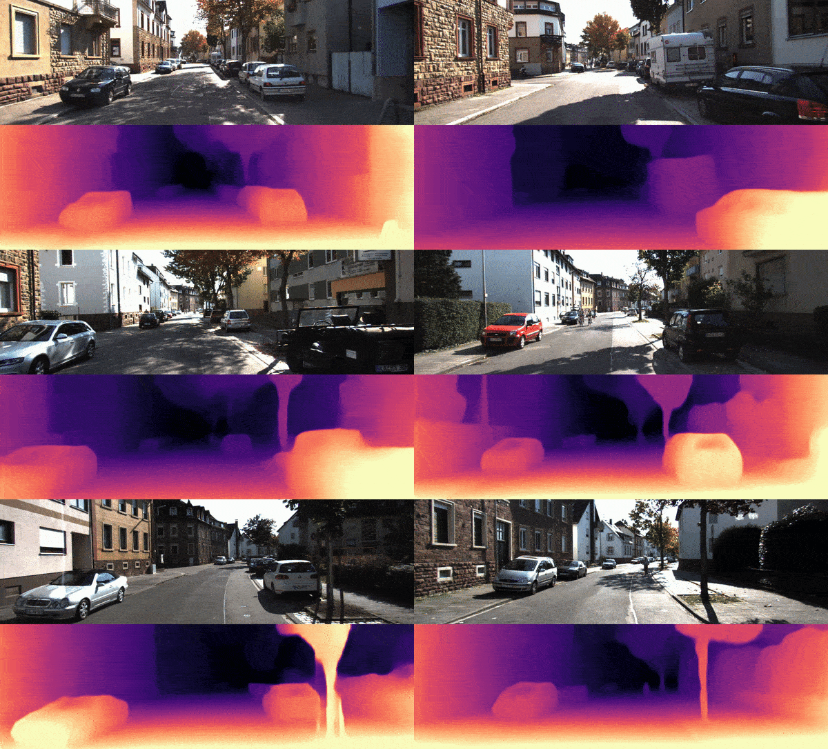
The result video for the example:

You can start with the example code.

Download the script to run the demo

Download cam_demo.py

This example command will load an image sequence then store a video:

python demo.py --model_zoo monodepth2_resnet18_kitti_mono_stereo_640x192 --input_format image --data_path ~/.mxnet/datasets/kitti/example/2011_09_26/2011_09_26_drive_0095_sync/image_02/data --output_format video

This example command will load an image sequence then store the corresponding colorized disparity sequence:

python demo.py --model_zoo monodepth2_resnet18_kitti_mono_stereo_640x192 --input_format image --data_path ~/.mxnet/datasets/kitti/example/2011_09_26/2011_09_26_drive_0095_sync/image_02/data --output_format image

For more demo command options, please run python demo.py -h

Hint

This tutorial directly loads the image sequence or video into a list, so it cannot work when the image sequence or video is large. Here is just provide an example about using a pretrained monodepth2 model to do a prediction for users.