1. Getting Started with Pre-trained Model on CIFAR10file_download

Download demo_cifar10.py

file_download

Download Python source code: demo_cifar10.py

file_download

Download Jupyter notebook: demo_cifar10.ipynb

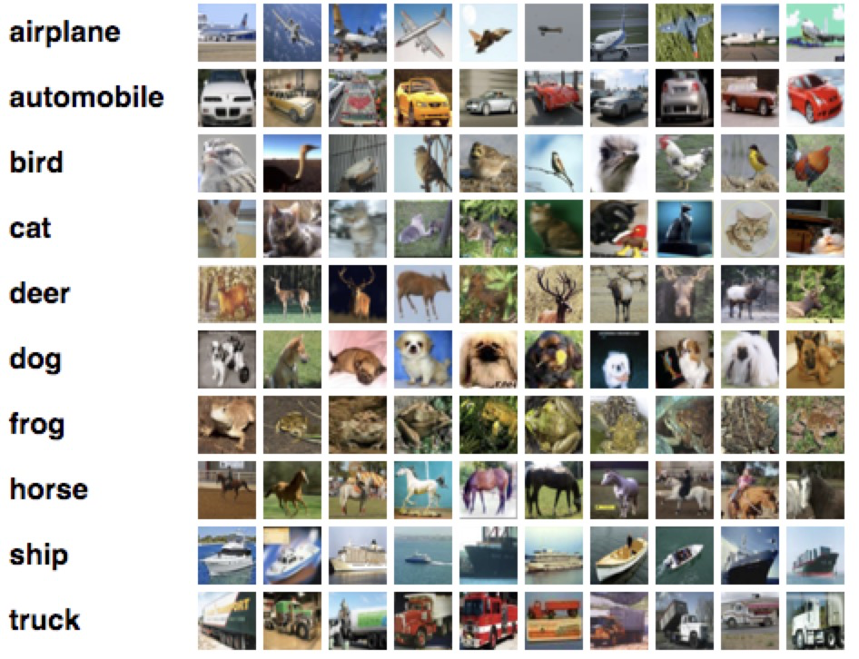
CIFAR10 is a dataset of tiny (32x32) images with labels, collected by Alex Krizhevsky, Vinod Nair, and Geoffrey Hinton. It is widely used as benchmark in computer vision research.

In this tutorial, we will demonstrate how to load a pre-trained model from gluoncv-model-zoo and classify images from the Internet or your local disk.

Step by Step

Let’s first try out a pre-trained cifar model with a few lines of python code.

First, please follow the installation guide to install MXNet and GluonCV if you haven’t done so yet.

import matplotlib.pyplot as plt

from mxnet import gluon, nd, image
from mxnet.gluon.data.vision import transforms
from gluoncv import utils
from gluoncv.model_zoo import get_model

Then, we download and show the example image:

url = 'https://raw.githubusercontent.com/dmlc/web-data/master/gluoncv/classification/plane-draw.jpeg'
im_fname = utils.download(url)

img = image.imread(im_fname)

plt.imshow(img.asnumpy())
plt.show()

Out:

Downloading plane-draw.jpeg from https://raw.githubusercontent.com/dmlc/web-data/master/gluoncv/classification/plane-draw.jpeg...

  0%|          | 0/99 [00:00<?, ?KB/s]
100%|##########| 99/99 [00:00<00:00, 20098.55KB/s]

In case you don’t recognize it, the image is a poorly-drawn airplane :)

Now we define transformations for the image.

transform_fn = transforms.Compose([
    transforms.Resize(32),
    transforms.CenterCrop(32),
    transforms.ToTensor(),
    transforms.Normalize([0.4914, 0.4822, 0.4465], [0.2023, 0.1994, 0.2010])
])

This transformation function does three things: resize and crop the image to 32x32 in size, transpose it to num_channels*height*width, and normalize with mean and standard deviation calculated across all CIFAR10 images.

What does the transformed image look like?

img = transform_fn(img)
plt.imshow(nd.transpose(img, (1,2,0)).asnumpy())
plt.show()

Can’t recognize anything? Don’t panic! Neither do I. The transformation makes it more “model-friendly”, instead of “human-friendly”.

Next, we load a pre-trained model.

net = get_model('cifar_resnet110_v1', classes=10, pretrained=True)

Out:

Downloading /root/.mxnet/models/cifar_resnet110_v1-a0e1f860.zip from https://apache-mxnet.s3-accelerate.dualstack.amazonaws.com/gluon/models/cifar_resnet110_v1-a0e1f860.zip...

  0%|          | 0/6335 [00:00<?, ?KB/s]
  2%|1         | 98/6335 [00:00<00:08, 724.72KB/s]
  8%|8         | 514/6335 [00:00<00:02, 2160.26KB/s]
 34%|###4      | 2179/6335 [00:00<00:00, 6939.53KB/s]
6336KB [00:00, 13047.08KB/s]

Finally, we prepare the image and feed it to the model

pred = net(img.expand_dims(axis=0))

class_names = ['airplane', 'automobile', 'bird', 'cat', 'deer',
               'dog', 'frog', 'horse', 'ship', 'truck']
ind = nd.argmax(pred, axis=1).astype('int')
print('The input picture is classified as [%s], with probability %.3f.'%
      (class_names[ind.asscalar()], nd.softmax(pred)[0][ind].asscalar()))

Out:

The input picture is classified as [airplane], with probability 0.393.

Play with the scripts

Here is a script that does all the previous steps in one go.

Feed in your own image to see how well it does the job. Keep in mind that CIFAR10 is a small dataset with only 10 classes. Models trained on CIFAR10 only recognize objects from those 10 classes. Thus, it may surprise you if we feed one image to the model which doesn’t belong to any of the 10 classes

For instance we can test it with the following photo of Mt. Baker:

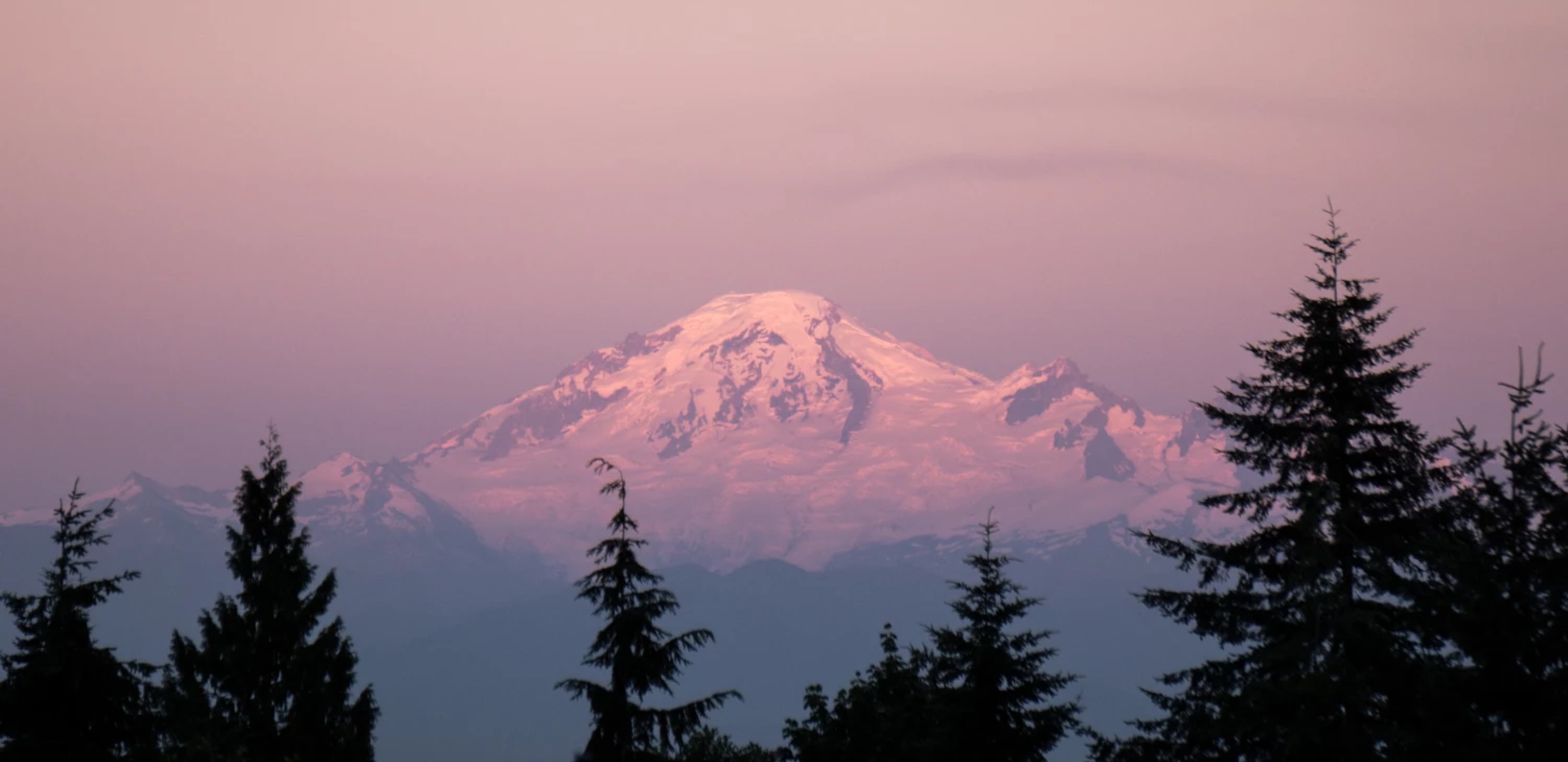
python demo_cifar10.py --model cifar_resnet110_v1 --input-pic mt_baker.jpg

The result is:

The input picture is classified to be [ship], with probability 0.949.

Next Step

Congratulations! You’ve just finished reading the first tutorial. There are a lot more to help you learn GluonCV.

If you would like to dive deeper into training on CIFAR10, feel free to read the next tutorial on CIFAR10.

Or, if you would like to try a larger scale dataset with 1000 classes of common objects please read Getting Started with ImageNet Pre-trained Models.